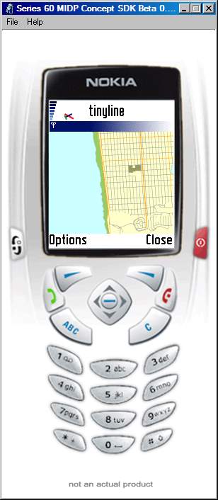
Figure 7: A fragment of San Diego area map in the TinyLine viewer
Keywords: mobile phone, AxioMap, SVG-Tiny, web services
Biography
Ilya Zaslavsky leads the Spatial Information Systems Lab at SDSC (San Diego Supercomputer Center) . His interests include GIS (Geographic Information Systems) , spatial databases, spatial data integration, and SVG (Scalable Vector Graphics) .
Biography
Ashraf Memon is the lead software architect for the Geosciences Network project at SDSC. He is an expert in web services and spatial databases.
Using SVG for rendering maps on mobile devices results in better graphic quality with reduced bandwidth requirements, while making it easier to display continuously moving objects and create maps from multiple sources. This paper describes our experience developing web services to generate SVG Tiny maps for mobile phones. The map information is largely derived from common ESRI (Environmental Systems Research Institute) ’s ArcIMS (Arc Internet Map Server) spatial data servers which are often used by federal and other agencies to provide public-domain street and other data. We present the composition of the web service, and the range of data transformation techniques for optimizing SVG document sizes and rendering speed.
1. Introduction
2. The Structure of the SVG Generator Service
3. Optimizations
3.1 Adjusting to screen size of target device
3.2 Trade-offs between interactivity and document size and organization
3.3 Concatenating path fragments
3.4 Line generalization
4. Conclusion
Acknowledgements
Bibliography
The mainstream approach to online mapping relies on GET_IMAGE, getmap or similar requests against Internet map servers that generate map images to be displayed at a mapping client. Limitations of this approach are well known: (1) it is not suitable for applications that require continuous map updates and/or high level of interactivity at the client; (2) it is bandwidth-intensive and places severe load on the map server, (3) it does not take advantage of increasing processing and graphics capabilities of map clients, and (4) it is not well suited for situations where data are drawn from multiple servers and need to be combined at the client. This last limitation is particularly apparent in mobile devices, where maps are composed of objects that “move with the device”, and map fragments that remain relatively stable and can be reused. For example, location of cell phone may be shown as a slowly moving dot with position updated by some location service (such as phone number-based lookup, or a connected GPS device) while the underlying street map may be updated only when the point approaches a map edge thus dramatically reducing the number of required map updates. SVG provides an excellent platform for such a client application.
With the growing acceptance of SVG Tiny and SVG Basic profiles [Mobile SVG] , and proliferation of Java-enabled or SVG -enabled mobile devices, SVG viewers and editors (e.g. reviewed at http://scale-a-vector.de/), the primary issue becomes creating the infrastructure of services for generation of on demand SVG maps accessible from the mobile phones. Ideally, this infrastructure would re-use existing spatial data services created for conventional Internet mapping. In this paper, we focus on SVG Tiny generation from common ArcIMS services, and describe the API and functionality of a working SVG generator capable of creating SVG maps for different types of client devices. The next section describes the structure and methods of the web service. It is followed by a discussion of data transformations needed for making SVG output more efficient.
The SVG generator service is written in Java and uses the Batik toolkit [BATIK] to create and manipulate an SVG document. SVG Tiny generation represents a sequence of service requests as shown in Table 1 . Note that these requests are formulated over an abstract XML coordinate data service, which may represent an ArcIMS image service capable of retrieving feature coordinates via GET_FEATURES request with geometry=true (provided that GET_FEATURES is not disabled in the service), or a WFS (Web Feature Service) returning GML (Geography Markup Language) , or similar. The examples below use ArcIMS image services as the most wide-spread at the time of writing.
Table 1 below lists methods of the SVG Generator web service, while the following code fragments provide implementation examples:
| get_capabilities | returns information about the XML coordinate data service, including the service’s spatial envelope, and a list and rendering information for all layers contained in the service (for ArcIMS sources, this request translates into ArcXML GET_SERVICE_INFO requests). |
| set_map | computes an optimal SVG coordinate system (which depends on the client pixel dimensions and anticipated interactivity), sets the map extent (either based on the map service’s spatial envelope, or information about the device location received from a location service or the device’s GPS receiver), and generates a sequence of calls against each layer to be included in the SVG map (based on the information returned in the previous request). |
| add_renderer | inserts rendering information for each layer into SVG <def> elements, derived from layer styling data (size, width, fill-color, outline-width, outline-color) retrieved by the get_capabilities request. |
| add_point_layer add_line_layer add_polygon_layer | for each requested vector layer, convert coordinate information received from an XML coordinate data service, and rendering information added in the add_renderer call, into a sequence of SVG <circle> or <rect> (for point layers), or <path> (for line and polygon layers) elements, and add layer groups to the SVG document. In case of ArcIMS services, the coordinate information is extracted from ArcIMS responses to GET_FEATURES requests. |
| add_labels | retrieves labeling information from the source, including label location and rotation, creates a sequence of SVG <text> elements and adds them to the SVG document. In case of ArcIMS sources, this information is retrieved from layers that include <SIMPLELABELRENDERER> element. |
| get_svg | returns the generated SVG document string specific for the requesting device. |
Table 1
To illustrate the operation of the service, consider several example requests, executed against ArcIMS image service named GDT_ArcWeb_US_SVG residing at arcwebdemo.esri.com. This service provides street information over a set of common base geographic layers, and includes: Oceans and Seas; U.S. Counties; Major Parks; Landmark Areas; Airports; Rivers and Streams; Water Bodies; Railroads; Streets; Highways U.S. Cities. In the experiments describe below, we focused on downtown area of San Francisco, around Moscone Convention Center (spatial envelope: minx = -122.60; maxx = -122.39; miny = 37.75; maxy = 37.79).
A GET_SERVICE_INFO request is used to retrieve the content of the service and layer schemas and rendering information; it returns the following ArcXML document ( Figure 1 ):
<?xml version="1.0" encoding="UTF-8"?> <ARCXML version="1.1"> <RESPONSE> <SERVICEINFO> <ENVIRONMENT> <LOCALE language="en" /><UIFONT name="Arial" color="0,0,0" size="12" style="regular" /> <SEPARATORS cs=" " ts=";"/><CAPABILITIES forbidden=""/> <SCREEN dpi="96"/><IMAGELIMIT pixelcount="1048576" /> </ENVIRONMENT> <PROPERTIES><ENVELOPE minx="-170" miny="16" maxx="-66" maxy="72" /> <MAPUNITS units="DECIMAL_DEGREES" /> <BACKGROUND color="255,255,255" /></PROPERTIES> <LAYERINFO type="featureclass" visible="true" name="Oceans and Seas" id="Oceans and Seas" minscale="0.000059486524036121"> <FCLASS type="polygon"> <ENVELOPE minx="-180" miny="-90" maxx="180" maxy="90" /> <FIELD name="MISC.ESRI_OCEAN1.AREA" type="8" size="15" precision="4" /> <FIELD name="MISC.ESRI_OCEAN1.PERIMETER" type="8" size="15" precision="4" /> <FIELD name="MISC.ESRI_OCEAN1.OCEAN1_" type="4" size="9" precision="0" /> <FIELD name="MISC.ESRI_OCEAN1.OCEAN1_ID" type="4" size="9" precision="0" /> <FIELD name="#SHAPE#" type="-98" size="0" precision="0" /> <FIELD name="MISC.ESRI_OCEAN1.OBJECTID" type="-99" size="16" precision="0" /> </FCLASS> <SIMPLERENDERER> <SIMPLEPOLYGONSYMBOL fillcolor="204,255,255" filltype="solid" boundary="false" /></SIMPLERENDERER> </LAYERINFO> . . . |
Figure 1: ArcXML response to a GET_SERVICE_INFO request against the sample service
Based on the information about the available layers, we can now formulate requests for coordinate data to each of them. All feature geometry requests are formulated in a similar manner, as in the following example requesting feature coordinates for the Rivers layer ( Figure 2 ):
<?xml version="1.0" encoding="UTF-8"?> <ARCXML version="1.1"> <REQUEST> <GET_FEATURES outputmode="newxml" geometry="true" envelope="true" compact="true"> <LAYER id="Rivers 4"/> <SPATIALQUERY subfields="#ALL#" where="" > <SPATIALFILTER relation="area_intersection"> <ENVELOPE minx="-122.60" miny="37.75" maxx="-122.39" maxy="37.79" /></SPATIALFILTER></SPATIALQUERY></GET_FEATURES> </REQUEST> </ARCXML> |
Figure 2: ArcXML feature geometry request
An ArcXML response to this request contains the following ( Figure 3 ):
<?xml version="1.0" encoding="UTF-8"?> <ARCXML version="1.1"> <RESPONSE> <FEATURES> <FEATURE> <ENVELOPE minx="-122.488372" miny="37.5" maxx="-122.009532" maxy="37.997842"/> <FIELDS> <FIELD name="#SHAPE#" value="[Geometry]" /> <FIELD name="GDT.MPF_WATER.CFCC" value="H11" /> <FIELD name="GDT.MPF_WATER.OBJECTID" value="3114" /> </FIELDS> <POLYLINE> <PATH> <COORDS>-122.113774 37.80272;-122.113912 37.802571</COORDS> </PATH> <PATH> <COORDS>-122.197835 37.799895;-122.197919 37.79947</COORDS> </PATH> . . . . . . |
Figure 3: ArcXML response with coordinate geometry of a line layer
ArcXML responses for polygon and point layers are slightly different. Polygon geometry is returned as in the following example ( Figure 4 ):
<?xml version="1.0" encoding="UTF-8"?> <ARCXML version="1.1"> <RESPONSE> <FEATURES> <FEATURE> <ENVELOPE minx="-122.497689" miny="37.74944" maxx="-122.495519" maxy="37.751544"/> <FIELDS> <FIELD name="GDT.GDT_AREALANDMARK_LG.GDT_ID" value="" /> <FIELD name="GDT.GDT_AREALANDMARK_LG.STATE_FIPS" value="6" /> <FIELD name="GDT.GDT_AREALANDMARK_LG.COUNTY_FIPS" value="75" /> <FIELD name="GDT.GDT_AREALANDMARK_LG.NAME" value="A P GIANNINI MIDDLE SCHOOL" /> <FIELD name="GDT.GDT_AREALANDMARK_LG.CFCC" value="D43" /> <FIELD name="#SHAPE#" value="[Geometry]" /> <FIELD name="GDT.GDT_AREALANDMARK_LG.OBJECTID" value="11433" /> </FIELDS> <POLYGON> <RING> <COORDS>-122.496741 37.751503;-122.496176 37.751524;-122.495674 37.751544;-122.49553 37.749687;-122.495519 37.749539;-122.497584 37.74944;-122.497636 37.750481;-122.497689 37.751454;-122.496741 37.751503</COORDS> </RING> </POLYGON> </FEATURE> . . . . . . |
Figure 4: ArcXML response with coordinate geometry of a polygon layer
while point geometry is returned using the MULTIPOINT construct ( Figure 5 ):
<ARCXML version="1.1"> <RESPONSE> <FEATURES> <FEATURE> <ENVELOPE maxx="-122.420242730756" maxy="37.7747196054092" minx="-122.420242730756" miny="37.7747196054092"/> <FIELDS> <FIELD name="ESRI.MD_PLACES_PT.FEATURE" value="Population 500,000 to 999,999 County Seat"/> <FIELD name="ESRI.MD_PLACES_PT.NAME" value="San Francisco"/> <FIELD name="ESRI.MD_PLACES_PT.FIPS" value="06075"/> <FIELD name="ESRI.MD_PLACES_PT.FIPS55" value="67000"/> <FIELD name="ESRI.MD_PLACES_PT.POP_CLASS" value="2"/> <FIELD name="ESRI.MD_PLACES_PT.AREA_CLASS" value="2"/> <FIELD name="ESRI.MD_PLACES_PT.STATE" value="California"/> <FIELD name="ESRI.MD_PLACES_PT.CAPITAL" value="3"/> <FIELD name="ESRI.MD_PLACES_PT.RANK" value="1"/> <FIELD name="ESRI.MD_PLACES_PT.POPULATION" value="723959"/> <FIELD name="#SHAPE#" value="[Geometry]"/> <FIELD name="ESRI.MD_PLACES_PT.ORANK" value="1"/> <FIELD name="ESRI.MD_PLACES_PT.OBJECTID" value="2014"/> </FIELDS> <MULTIPOINT> <COORDS>-122.420242730756 37.7747196054092</COORDS> </MULTIPOINT> </FEATURE> <FEATURECOUNT count="1" hasmore="false"/> </FEATURES> </RESPONSE> </ARCXML> |
Figure 5: ArcXML response with coordinate geometry of a point layer
Now that we have the map’s spatial extent and layer drawing sequence, as well as coordinate and rendering information for each layer, we are ready to convert this information into an SVG Tiny document, as in the following example ( Figure 6 ):
<?xml version="1.0" standalone="no" ?> <!DOCTYPE svg PUBLIC "-//W3C//DTD SVG 1.1 Tiny//EN" "http://www.w3.org/Graphics/SVG/1.1/DTD/svg11-tiny.dtd"> <svg contentScriptType="text/ecmascript" width="100%" xmlns:xlink="http://www.w3.org/1999/xlink" baseProfile="tiny" zoomAndPan="magnify" contentStyleType="text/css" id="svg-root" height="100%" preserveAspectRatio="xMidYMid meet" xmlns="http://www.w3.org/2000/svg" version="1.1"> <defs> <circle fill="#ffff99" r="180.0" cx="0" cy="0" id="renderer_U.S. Cities" stroke="none" stroke-width="1"/> </defs> <g id="karta" transform="scale(0.048761904761906213,-0.048761904761906213) translate(0,-4000)"> <g id="polygons"> <path fill="#ccffff" stroke-width="1" id="Oceans and Seas" d="M30260000,-12775000L-5740000,-12775000 -5740000,5225000 30260000,5225000 30260000,-12775000 z " stroke="none"/> |
Figure 6: Fragment of an SVG Tiny document converted from ArcXML responses
The service thus generates an SVG Tiny-compliant document suitable for rendering on J2ME-enabled cell phones (using TinyLine [TinyLine] in particular, as in Figure 7 ). However, before the SVG Tiny document from the service can be sent to a mobile device, several optimizations must be performed, as described in the following section.
The total size of ArcXML documents containing rendering and geometry information retrieved from the GDT_ArcWeb_US_SVG service within the given envelope, is 1,435,454 bytes, while the SVG Tiny document generated from the ArcXML responses is 1,092,407 bytes. This size is not acceptable for the current generation of mobile clients and transmission speeds. This section describes several geometric manipulations for reducing the size of SVG documents and optimizing DOM. Optimizations are different for different types of target devices. To some extent, the techniques described here, inherit from an earlier system called AxioMap (Application of XML for Interactive Online Mapping) [AxioMap] , which was presented at the SVG Open 2002 in Zurich [AxioMap SVGOpen Paper] .
To improve rendering speed, the service establishes a false map origin, and converts feature coordinates to a local SVG coordinate space transforming coordinate values into integers (3-digit integers for small-screen devices, 4-5-digit integers for desktop). The conversion details are given in [AxioMap SVGOpen Paper] . In our sample service, conversion to 5-digit integers resulted in significant file size savings (from 1,092,407 bytes before conversion down to 622,676 bytes), with minor increase in processing time (from 16046ms to 16219 ms).
Typically, converting ArcXML polygon and polyline feature coordinates into SVG , we map features to individual SVG path elements. However, SVG renderers are known to be more efficient when the count of objects in DOM is smaller, despite the increased size of individual objects. Indeed, identity of individual features in a layer may not be important if the layer is not likely to be queried, or a client device does not support scripting / mouse events (as in the case of the canonical SVG Tiny).
To take advantage of this circumstance, the SVG generator creates a particular flavor of SVG Tiny (i.e. with geometric features individually mapped into path statements within a layer group, or with all features in a layer combined into a single path), depending on the signature of the requesting client. Concatenating individual features into a single path results in file size improvements between 10-20%, in our experiments, at the same time dramatically reducing counts of objects in the SVG document.
Usually, line data served by online services, are far from optimal for SVG . As an artifact of digitizing or coordinate conversion, a line feature may consist of multiple fragments arranged in mysterious order and pointing in different directions. (This could be especially overwhelming if we decide to convert all features in a line layer into a single path as described above).
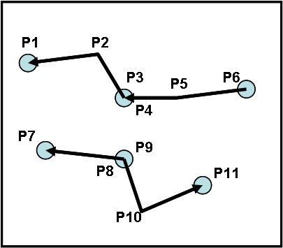
Suppose, that the initial path ( Figure 8 ) is described as:
d="M x3,y3 L x2,y2 x1,y1 M x6,y6 L x5,y5 x4,y4 M x8,y8 L x7,y7 M x9,y9 L x10,y10 x11,y11"
Obviously, the same information can be presented more efficiently:
d="M x6,y6 L x5,y5 x3,y3 x2,y2 x1,y1 M x7,y7 L x8,y8 x10,y10 x11,y11"
if the path fragments are concatenated into two fragments instead of the initial four. We developed a simple one-pass (after sorting) algorithm that reduces the number of path fragments by concatenating them into longer fragments. The algorithm:
In our experiments with Moscone area service, concatenating path fragments reduced the size of SVG files by 5-7% on average. The street layer appears initially tighter (i.e. with shorter line chains per feature), thus average gain from concatenating street layers is smaller (about 4.8%). However, if line features are assembled into a limited number of paths per layer, concatenation of fragments results in a much better improvement. For example, concatenating path fragments of the streets layer in another service named svg_esri at http://geo.sdsc.edu resulted in 51.6% document size reduction. The reason is that the street layer in that service was based on Tiger 2000 files with many unnamed street segments in the area, and that the street features had been merged on street name (in ArcView, prior to serving on the Internet). This resulted in a single large path containing all unnamed street segments. Concatenating fragments of this path largely contributed to the increased efficiency.
Finally, we applied the Douglas-Poiker line simplification algorithm [Douglas-Poiker] to further tighten SVG Tiny output. The algorithm is well known, and Java code implementing it is available on the Web [Douglas-Poiker Java] , so we don’t provide algorithm details in this paper.
Overall, applying the sequence of optimization routines described above reduced the size of the SVG document by more than 3 times (from 1,092,407 bytes down to 341,455), without any visible change in geometry and significant increase in processing time (16046 ms for generating initial SVG Tiny from ArcXML documents; 16281 ms for generating an optimized version).
Figure 9 and Figure 10 show a fragment of a San Francisco SVG map generated from the GDT_ArcWeb_US_SVG service, before and after the optimizations, in the TinyLine [TinyLine] SVG Viewer
Displaying SVG maps on mobile devices is difficult because maps often contain large amounts of graphic information, while mobile devices (phones, PDAs) have limited processing and rendering capabilities. Additional difficulty is that geographic data available on demand from multiple mapping services, are not optimized for SVG . Addressing this challenge, we demonstrated a web service for generating SVG Tiny maps from widely available Internet map servers, and discussed a range of optimization techniques aimed at decreasing the size of the map documents and restructuring them for faster rendering. The SVG maps were tested and display correctly in Adobe’s, Squiggle and TinyLine SVG viewers.
The described service is a work in progress. Its current limitations include inability to translate complex ArcXML rendering instructions (including VALUEMAPRENDERER, SCALEDEPENDENTRENDERER, SIMPLELABELRENDERER, GROUPRENDERER tags, specification of point symbols, and several other instructions common in ArcXML configuration files.) These limitations will be addressed in the next version.
This work is partially funded by ESRI and a University of California Discovery grant.
XHTML rendition created by gcapaper Web Publisher v2.1, © 2001-3 Schema Software Inc.